ChIP-seq

Preprocessing of ChIP-seq has never been easier!

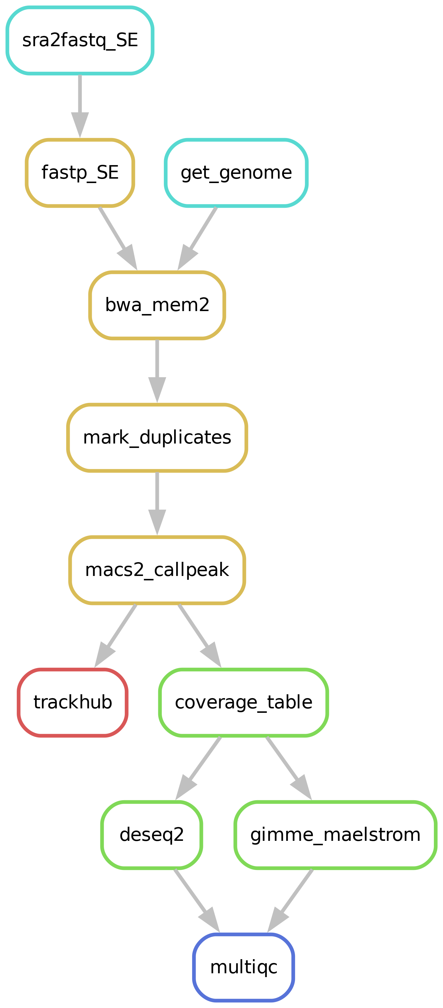
Workflow overview (simplified)

An example quality control report can be viewed here.

Downloading of sample(s)

Depending on whether the samples you start seq2science with is your own data, public data, or a mix, the pipeline might start with downloading samples. The downloading of samples is integrated into each workflow, so you don’t have to start a download workflow first. You control which samples are used in the samples.tsv. Background on public data can be found here.

Downloading and indexing of assembly(s)

Depending on whether the assembly and its index you align your samples against already exist seq2science will start with downloading of the assembly through genomepy.

Read trimming

The pipeline starts by trimming the reads with Trim Galore! or Fastp (the default). The trimmer will automatically trim the low quality 3’ ends of reads, and removes short reads. During quality trimming it automatically detects which sequencing adapter was used (if it wasn’t trimmed off yet), and then trims this as well. Trimming parameters for the pipeline can be set in the configuration, for example:

trimmer:
  fastp:
    trimoptions: --trim_front1 3 --trim_front2 14 --trim_poly_x

Alignment

After trimming the reads are aligned against an assembly. Currently we support bowtie2, bwa, bwa-mem2, hisat2, minimap2 and STAR as aligners. Choosing which aligner is as easy as setting the aligner variable in the config.yaml, for example: aligner: bwa. Sensible defaults have been set for every aligner, but can be overwritten for either (or both) the indexing and alignment by specifying them in the config.yaml:

aligner:
  bwa-mem:
    index: '-a bwtsw'
    align: '-M'

The pipeline will check if the assembly you specified is present in the genome_dir, and otherwise will download it for you through genomepy. All these aligners require an index to be formed first for each assembly, but don’t worry, the pipeline does this for you.

Bam sieving

After aligning the bam you can choose to remove unmapped reads, low quality mappings, duplicates, and multimappers.

Peak calling

Currently we support two peak callers for the ChIP-seq workflow, MACS2 and genrich.

MACS2

MACS2 is the successor of MACS, created by taoliu (also one of the co-authors of hmmratac). MACS2 generates a ‘pileup‘ of all the reads. You can imagine this pileup as laying all reads on top of each other on the genome, and counting how high your pile gets for each basepair. MACS2 then models ‘background‘ values, based on the total length of all your reads and the genome length, to a Poisson distribution and decides whether your experimental pileup is significant compared to the poisson distribution. MACS2 is one of the, if not the, most used peak caller.

For the calculation of peaks MACS2 requires that an “effective” genome size is being passed as one of its arguments. For the more common assemblies (e.g. mm10 and human) these numbers can be found online. However we found googling these numbers quite the hassle, and for lesser studied species these numbers can’t be found online. Therefore the pipeline automatically estimates the effective genome size, we calculate this as the number of unique kmers of the average read length.

Broad peaks

The MACS2 peak caller also supports broad peak calling, and so does seq2science. To let MACS2 call broad peaks you have to add --broad to the macs2 command, e.g.:

peak_caller:
  macs2:
      --keep-dup 1 --broad

Genrich

Genrich is a spiritual successor of MACS2, created by John M. Gaspar. Just like MACS2 is generates a ‘pileup’. However the author of genrich realized that the distribution of pileup never follows a poisson distribution. Genrich then uses a log-normal distribution to model the background.

Quality report

It is always a good idea to check the quality of your samples. Along the way different quality control steps are taken, and are outputted in a single multiqc report in the qc folder. Make sure to always check the report, and take a look at interpreting the multiqc report!

Count table

A useful result the pipeline outputs is the count table, located at {counts_dir}/{peak_caller}/. For each narrowpeak (across all samples) its summit is taken, and all other summits within range peak_windowsize (default 100) are taken together, and the summit with the highest q-value is taken as the “true” peak. The remaining peaks are extended by slop on each side and for each sample the number of reads are counted under this peak. This file is stored as {assembly}_raw.tsv, and looks something like this:

                sample1     sample2
chr1:5649-5849  75.00000    0.00000
chr1:7399-7599  47.00000    1.00000

Note: since peaks are combined on their summit, NO count table is outputted for broad peaks.

Seq2science currently supports four different normalisation methods: quantile normalisation, TMM, RLE, and upperquartile normalisation, and does count-per-million (counts under peaks) normalisation on each before normalisation.

**Quantile normalization** is a type of normalization that makes the distribution between samples identical. This means that the actual count distribution within a sample changes. This normalisation is especially powerful when comparing results from different labs/experiments/experimental methods.
TMM is the weighted trimmed mean of M-values proposed by Robinson and Oshlack (2010).
RLE is the scaling factor method proposed by Anders and Huber (2010). DEseq2’s standard normalisation is based on this.
Upper quartile is the upper-quartile normalization method of Bullard et al (2010).

After these normalisations the counts are log normalised, and the base can be set with logbase and defaults to 2. As a final step the count tables are mean-centered. Note that this table contains all peaks, and no selection on differential peaks has been made.

Differential motif analysis

Seq2science supports differential motif analysis! This analysis is based on the tool gimme maelstrom. As input to gimme maelstrom is the log 2 transformed quantile normalized count table of the biological reps (average between reps) in the consensus peakset. It then tries to solve a system of linear equations, where the output is the read counts in a peak, and the input is the motif score in the peak times the “motif activity”. This motif activity can then be compared across biological replicates for differential motifs.

By default seq2science makes use of the gimme.vertebrate.v5.0 motif database. This can be changed with the gimme_maelstrom_database config option. The gimme.vertebrate.v5.0 motif database is based on human and mouse gene names. When making use of a non-human/mouse genome assembly, seq2science makes use of the gimme motif2factors command to update the gene names for the used assembly. This option can be turned on/off with the infer_motif2factors option. Updating the motif database is done by downloading a set of other genome assemblies (including mouse and human), and inferring the orthologous between the used assembly and the human/mouse motif database. The config option motif2factors_reference controls which assemblies are used for ortholog inference, and comes with a default set of vertebrate assemblies. The config option motif2factors_database_references controls on which assemblies the reference is based on, and is by default the human and mouse genome assembly.

If you change the gimme_maelstrom_database to, for instance, an invertebrate database, and you want the motif database to use the gene names in your assembly. You will also have to update the motif2factors_reference and the motif2factors_database_references.

See the gimme motif2factors docs for a more extensive explanation of how the motif database is updated.

Differential peak analysis

On top of that, Seq2science can also use the raw peak counts table to perform differential peak analysis with DESeq2. See the Differential gene/peak analysis page for more information!

Trackhub

A UCSC compatible trackhub can be generated for this workflow. See the trackhub page for more information!

Filling out the samples.tsv

Before running a workflow you will have to specify which samples you want to run the workflow on. Each workflow starts with a samples.tsv as an example, and you should adapt it to your specific needs. As an example, the samples.tsv could look something like this:

sample    assembly    replicate    descriptive_name    control
GSM123    GRCh38      heart_1      heart_merged        GSM234
GSM321    GRCh38      heart_1      heart_merged        GSM234
GSMabc    GRCh38      heart_2      heart_not_merged    GSM234
GSMxzy    danRer11    stage_8      stage_8             GSM234
GSM890    danRer11    stage_9      stage_9             GSM234

Sample column

If you use the pipeline on public data this should be the name of the accession (e.g. GSM2837484). Accepted formats start with “GSM”, “SRR”, “SRX”, “DRR”, “DRX”, “ERR” or “ERX”.

If you use the pipeline on local data this should be the basename of the file without the extension(s). For example:

/home/user/myfastqs/sample1.fastq.gz ——-> sample1 for single-ended data
/home/user/myfastqs/sample2_R1.fastq.gz ┬> sample2 for paired-ended data
/home/user/myfastqs/sample2_R2.fastq.gz ┘

For local data, some fastq files may have slightly different naming formats. For instance, Illumina may produce a sample named sample3_S1_L001_R1_001.fastq.gz (and the R2 fastq). Seq2science will attempt to recognize these files based on the sample name sample3.

For both local and public data, identifiers used to recognize fastq files are the fastq read extensions (R1 and R2 by default) and the fastq suffix (fastq by default). The directory where seq2science will store (or look for) fastqs is determined by the fastq_dir config option. In the example above, the fastq_dir should be set to /home/user/myfastqs. These setting can be changed in the config.yaml.

Assembly column

Here you simply add the name of the assembly you want your samples aligned against and the workflow will download it for you.

Control (input) column

In the control column you can (optionally) add the “sample name” of the input control. It is generally a bad idea to add the input control as a sample in the sample since generally peak callers fail on these samples. Doing so looks like this:

sample    assembly    control
GSM123    GRCh38      GSMabc

Descriptive_name column

The descriptive_name column is used for the trackhub and multiqc report. In the trackhub your tracks will be called after the descriptive name, and in the multiqc report there will be a button to rename your samples after this column. The descriptive name can not contain ‘-’ characters, but underscores ‘_’ are allowed.

technical_replicates column

Technical replicates, or any fastq file you may wish to merge on the fastq level, are set using the technical_replicates column in the samples.tsv file. All samples with the same name in the technical_replicates column will be concatenated into one file with the replicate name.

Example samples.tsv utilizing replicate merging:

sample    assembly    technical_replicates
GSM123    GRCh38      heart
GSMabc    GRCh38      heart
GSMxzy    GRCh38      stage8
GSM890    GRCh38

Using this file in the alignment workflow will output heart.bam, stage8.bam and GSM890.bam. The MultiQC will inform you of the trimming steps performed on all samples, and subsequent information of the ‘replicate’ files (of which only heart is merged).

Note: If you are working with multiple assemblies in one workflow, replicate names have to be unique between assemblies (you will receive a warning if names overlap).

keep

Replicate merging is turned on by default. It can be turned off by setting technical_replicates in the config.yaml to keep.

Biological replicates

During ATAC-seq workflows, peak calling can be performed per biological condition, depending on your configuration setting. Biological conditions are determined by the biological_replicates column in the samples.tsv file. How these samples are handled is specified by configuration variable biological_replicates.

sample    assembly    biological_replicates
GSM123    GRCh38      kidney
GSMabc    GRCh38      liver
GSMxzy    GRCh38      liver
GSM890    GRCh38

In this case peaks of the two liver samples (GSMabc and GSMxzy) will be combined by e.g. IDR.

Keep

By setting biological_replicates to keep, all biological replicates are analyzed individually. The biological_replicates column is ignored.

Irreproducible Discovery Rate (IDR)

One of the more common methods to combine biological replicates is by the irreproducible discovery rate (idr). Shortly; idr sorts all the peaks of two replicates separately on their significance. Since true peaks should be very significant for both replicates these peaks will be one of the highest sorted peaks. As peaks get less and less true (and thus their significance) their ordering also becomes more random between the samples. The idr method then only keeps the peak that overlap nonrandomly between the samples. The idr method only works for two replicates, so can not be used when you have more than 2. IDR can be turned on by setting biological_replicates to idr.

Fisher’s method

Fisher’s method simply is a method to ‘combine’ multiple p-values. This method is built-in for genrich and macs2, and allows any number of replicates (n >= 2). However a ‘disadvantage’ of this method is that it assumes the p-values a method generates are actual p-values (and not a general indication of significance). MACS2 is slightly notorious for that its p-values are not true p-values. Genrich claims by fitting on a log-normal distribution that their p-values are true. Even though fisher’s method might not be ideal, it’s the only option you have (we provide) within this pipeline for more than 2 replicates. Fisher’s method can be turned on by setting biological_replicates to fisher.

A mix of biological and technical replicates

sample    assembly    technical_replicates  biological_replicates
GSM123    GRCh38      peter_kidney         kidney
GSMabc    GRCh38      peter_liver          liver
GSMxzy    GRCh38      lindsey_liver        liver
GSM890    GRCh38      lindsey_liver        liver

In this example we have data from Peter and Lindsey. We have one liver sample and one kidney sample from Peter. Of Lindsey we only have a liver sample, which was sequenced across two different lanes. With this sample sheet, the samples of Lindsey get merged after trimming. Then peak calling is done separately on each of the three remaining technical replicates (peter_kidney, peter_liver, lindsey_liver), and afterwards all liver technical replicates belonging to the same biological replicate (in this case peter_liver and lindsey_liver) are combined through e.g. IDR.

Colors column

If you are visualizing your data on the UCSC trackhub you can optionally specify the colors of each main track. For ATAC- and ChIP-seq, each biological replicate is a main track. To do so, you can add the color by name (google “matplotlib colors” for the options), or RGB values, in the “colors” column. Empty fields are considered black.

Final notes

Make sure that the samples.tsv is a tab separated values file when running the pipeline.
Feel free to delete or add columns to your liking.

Filling out the config.yaml

Every workflow has many configurable options, and can be set in the config.yaml file. In each config.yaml we highlighted a couple options that we think are relevant for that specific workflow, and set (we think) reasonable default values.

When a workflow starts it prints the complete configuration, and (almost) all these values can be added in the config.yaml and changed to your liking. You can see the complete set of configurable options in the extensive docs.

Best practices

Irreproducible Discovery Rate

For idr to work properly, it needs a large portion of peaks that are actually not true peaks. Therefore we recommend to call peaks ‘loosely’. One way of doing this is setting the peak threshold q-value low for macs2 in the configuration. The q-value controls the ratio of false positives / (false positives + true positives). Setting a q-value of 1 guarantees you have plenty of false positives in your dataset for IDR to work properly.

subsampling

In some cases you might want to have the same number of reads between samples. By adding e.g. subsample:1_000_000 seq2science will make sure that each sample contains at most a million reads. Seq2science always downsamples, never upsamples.