scRNA-seq

Preprocessing of scRNA-seq has never been easier!

Workflow overview (simplified)

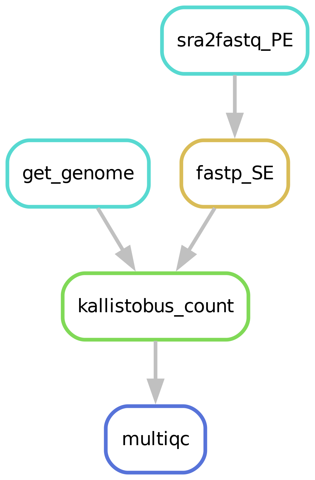
Downloading of sample(s)

Depending on whether the samples you start seq2science with is your own data, public data, or a mix, the pipeline might start with downloading samples. You control which samples are used in the samples.tsv. Background on public data can be found here.

Downloading and indexing of assembly(s)

Depending on whether the assembly and its index you align your samples against already exist seq2science will start with downloading of the assembly through genomepy.

Read trimming

The pipeline starts by trimming the reads with fastp. Fastp automatically detects sequencing adapters, removes short reads and performs quality filtering. The parameters of fastp for the pipeline can be set in the configuration by the variable fastp.

Note: fastp currently runs in single-end mode even if you provide paired-end fastq files. This is due to the fact that reads, barcode and umi sequences are stored in separate fastq files. After trimming, the fastq containing the reads, usually R2, may contains less reads then R1. Therefore, we perform an intermediate step by running fastq-pair to remove singleton reads before proceeding any further.

Quantification

Quantification is performed by running either the kb-python wrapper for Kallisto bustools or CITE-seq-Count for ADT tags. Kallisto bustools relies on pseudo-alignment of scRNA reads against a reference transcriptome index. The resulting count matrices can be further processed with scRNA toolkits, such as Seurat or Scanpy.

Filling out the samples.tsv

Before running a workflow you will have to specify which samples you want to run the workflow on. Each workflow starts with a samples.tsv as an example, and you should adapt it to your specific needs. As an example, the samples.tsv could look something like this:

sample  assembly        descriptive_name
pbmc    GRCh38.p13      pbmc

Sample column

If you use the pipeline on public data this should be the name of the accession (e.g. GSM2837484). Accepted formats start with “GSM”, “SRR”, “SRX”, “DRR”, “DRX”, “ERR” or “ERX”.

If you use the pipeline on local data this should be the basename of the file without the extension(s). For example:

• /home/user/myfastqs/sample1.fastq.gz ——-> sample1 for single-ended data

• /home/user/myfastqs/sample2_R1.fastq.gz ┬> sample2 for paired-ended data
  /home/user/myfastqs/sample2_R2.fastq.gz ┘

For local data, some fastq files may have slightly different naming formats. For instance, Illumina may produce a sample named sample3_S1_L001_R1_001.fastq.gz (and the R2 fastq). Seq2science will attempt to recognize these files based on the sample name sample3.

For both local and public data, identifiers used to recognize fastq files are the fastq read extensions (R1 and R2 by default) and the fastq suffix (fastq by default). The directory where seq2science will store (or look for) fastqs is determined by the fastq_dir config option. In the example above, the fastq_dir should be set to /home/user/myfastqs. These setting can be changed in the config.yaml.

Assembly column

Here you simply add the name of the assembly you want your samples aligned against and the workflow will download it for you. In case your intend to run kb-python’s kite workflow, the assembly name becomes the basename of the tab delimited feature barcode file.

Descriptive_name column

The descriptive_name column is used for the multiqc report. In the multiqc report there will be a button to rename your samples after this column.

Filling out the config.yaml

Every workflow has many configurable options, and can be set in the config.yaml file. In each config.yaml we highlighted a couple options that we think are relevant for that specific workflow, and set (we think) reasonable default values.

Custom assembly extensions

The genome and/or gene annotation can be extended with custom files, such as ERCC spike-ins for scRNA-seq. To do so, add custom_genome_extension: path/to/spike_in.fa and custom_annotation_extension: path/to/spike_in.gtf to the config. Seq2science will place the customized assembly in a separate folder in the genome_dir. You can control the name of the customized assembly by setting custom_assembly_suffix in the config.

Quantification with kallistobus

After initializing your working directory and editing the samples.tsv file, specify the desired arguments for kb-pyhon via the ref (kb ref) and count (kb count) properties except for the barcode whitelist (-w). The path to the barcode whiltelist can be supplied via the barcodefile property. This step is optional since kb python python provides several pre-installed whitelists for the following technologies.

• 10XV1

• 10XV2

• 10XV3

• INDROPSV3

The white-list will be installed automatically if the appropiate technology argument is provided via the -x parameter in short-hand syntax.

BUS (Barcode/UMI/Set) format

The -x argument indicates the read and file positions of the UMI and barcode. Kallisto bustools should auto-detect the correct settings barcode/umi layout for the following technologies if the name is supplied:

name         whitelist    barcode                  umi        cDNA
---------    ---------    ---------------------    -------    -----------------------
10XV1        yes          0,0,14                   1,0,10     2,None,None
10XV2        yes          0,0,16                   0,16,26    1,None,None
10XV3        yes          0,0,16                   0,16,28    1,None,None
CELSEQ                    0,0,8                    0,8,12     1,None,None
CELSEQ2                   0,6,12                   0,0,6      1,None,None
DROPSEQ                   0,0,12                   0,12,20    1,None,None
INDROPSV1                 0,0,11 0,30,38           0,42,48    1,None,None
INDROPSV2                 1,0,11 1,30,38           1,42,48    0,None,None
INDROPSV3    yes          0,0,8 1,0,8              1,8,14     2,None,None
SCRUBSEQ                  0,0,6                    0,6,16     1,None,None
SURECELL                  0,0,6 0,21,27 0,42,48    0,51,59    1,None,None
SMARTSEQ                                                      0,None,None 1,None,None
`

Alternatively, the layout can be specified as a bc:umi:set triplet. The first position indicates the read, the second position the start of the feature and the third position the end of the feature. For more information and examples on the BUS format, consider the Bus section in the Kallisto manual.

Input preparations for KITE workflow

The steps to prepare a scRNA analysis for Feature Barcoding experiments deviates slighlty from the standard seq2science workflow. In essence, we quantify the abundance of sequence features, such as antibody barcodes, rather than a set of transcripts for a certain species. Therefore, our index does not rely on a particular assembly but is build from these sequence features. Please consider the offical kite documentation for more details.

1. Prepare a two-column, tab-delimited file with your feature barcode in the first column and feature names in the second.

Example

sequence	name
AACAAGACCCTTGAG	barcode 1
TACCCGTAATAGCGT	barcode 2

We save this file as fb.tsv.

2. Copy this file to the genome folder specified in config.yaml where seq2science searches for assemblies.

3. Add the basename of the feature barcode tabel, in this case fb, to the assembly column in your samples.tsv file.

sample  assembly
pbmc    fb

An example of configuring kb-python for feature barcode analysis is shown below. Add the appropiate settings to your config.

Examples

RNA Quantification (10XV3)

quantifier:
  kallistobus:
    count: '-x 10xv3 --h5ad --verbose'

RNA velocity (CEL-Seq2)

quantifier:
  kallistobus:
    ref: '--workflow lamanno'
    count: '-x 1,8,16:1,0,8:0,0,0 --h5ad --verbose --workflow lamanno'

barcodefile: "1col_barcode_384.tab"

The RNA velocity workflow produces count matrices for unspliced/spliced mRNA counts.

KITE feature barcoding (CEL-Seq2)

quantifier:
  kallistobus:
    ref: '--workflow kite'
    count: '-x 1,8,16:1,0,8:0,0,0 --h5ad --verbose --workflow kite'

barcodefile: "1col_barcode_384.tab"

Quantification with CITE-seq-Count

CITE-seq-Count count can be used as an alternative quantifier to pre-process ADT/Cell-hashing experiments and generate read/umi count matrices. This option cannot be used in conjunction with kallistobus.

To enable quantification with CITE-Seq-count, add the following section to your config file

Example

quantifier:
  citeseqcount:
    count: '-cbf 9 -cbl 16 -umif 1 -umil 8 -cells 372 --max-error 1 --bc_collapsing_dist 1 --umi_collapsing_dist 1  -T 10 --debug'

barcodefile: "barcodes.tab"

scRNA-seq pre-processing and quality control

The seq2science scRNA workflow provides the option to perform automated pre-processing of raw scRNA-seq UMI count matrices. This is achieved by incorporating several quality control steps from the singleCellTK Bioconductor package, such as cell-calling, doublet detection and assessment of cell-wise mitochondrial RNA content.

The QC results are reported in comprehensive R Markdown reports and processed UMI count matrices are stored as SingleCellExperiment S4 objects. Any sample level metadata that has been added to the samples.tsv file will be transferred to the colData slot of the corresponding object and assigned to each cell identifier.

After running seq2science, these objects can be directly imported into R with the readRDS function for further down-stream analysis with your favorite R packages.

To perform scRNA-seq pre-processing, add the following section to your seq2science config.yaml. In this example, we pre-process a plate-based experiment from human tissue.

sc_preprocess:
   export_sce_objects: False
   run_sctk_qc: True
   sctk_data_type: cell
   use_alt_expr: False
   alt_exp_name: ""
   alt_exp_reg: ""
   sctk_mito_set: human-ensembl
   sctk_detect_mito: True
   sctk_detect_cell: False
   sctk_cell_calling: Knee

To enable the sctk_qc workflow, set run_sctk_qc=True. Alternatively, one can skip quality control and export the UMI count matrix to a SingleCellExperiment object by setting export_sce_objects=True. However, there is no need to set export_sce_objects manually when run_sctk_qc is enabled.

Next, select the type of UMI count matrix with the sctk_data_type parameter. Valid options are either cell or droplet, depending on the type of experiment.

• droplet
  The UMI count matrix contains empty droplets. These empty droplets will be removed (cell calling) before further processing.

• cell
  The UMI count matrix does not contain empty droplets but has not been processed yet.

We do not perform any gene/cell level filtering, except for empty droplets that are considered ambient RNA.

Advanced settings

To perform additional (optional) QC steps, consider the following parameters:

• sctk_detect_mito (default: True)
  Quantify the percentage of mitochondrial RNA for each cell.

• sctk_mito_set (default: human-ensembl)
  The mitochondrial gene set to use for quantification with syntax [human,mouse]-[ensembl,entrez,symbol]. At the moment, only human and mouse gene annotations are supported. This option is only considered when sctk_detect_mito=True.

• sctk_detect_cell (default: True)
  Perform cell-calling for droplet based experiments. Empty droplets will not be removed if set to False.

• sctk_cell_calling (default: Knee)
  Method used for cell calling with DropletUtils, either Knee or EmptyDrops. By default, EmptyDrops will use an FDR of 0.01 to identify empty droplets. If no option is provided, the inflection point will be used for cell calling. This option is only considered when sctk_detect_cell=True.

• sctk_export_formats: (default: ["Seurat"])
  List of file formats to export SingleCellExperiment objects. Valid options are Seurat, FlatFile and AnnData. Raw and processed sce objects will be exported to rds format by default.
  

• sctk_qc_algos: (default: ["QCMetrics", "scDblFinder", "decontX"])
  List of QC algorithms for runCellQC’s algorithm parameter.
  

• velo assay: (default: spliced)
  The assay to use for exporting and QC when kb is run in velocity mode with --workflow lamanno parameter. Valid options are either spliced or unspliced.

Alternative experiments

Information about alternative sequencing features, such as ERCC spike-ins, can be provided as an alternative experiment. An alternative experiment will be stored within the same SingleCellExperiment object as the main experiment but processed separately. To process alternative experiments, set the following options:

• use_alt_expr (default: False)
  Set to True if you wish to process alternative experiments.

• alt_exp_name (default: "")
  The name/title of the alternative experiment. This option is only considered if use_alt_expr=True.

• alt_exp_reg (default: "")
  Regular expression to filter alternative features from main experiment (.i.e,; "ERCC-*"). This option is only considered when use_alt_expr=True.

A previous addition of alternative features to the genome assembly (see section on custom assembly extensions) is a prerequisite.

Output files

After running the scRNA QC workflow, the output can be found in the following locations:

path/to/results/scrna-preprocess/{quantifier}/export:
This folder contains the exported raw SingleCellExperiment object, without any QC applied.

path/to/results/scrna-preprocess/{quantifier}/sctk:
This folder contains the QC reports and exported SingleCellExperiment object, divided into several subfolders and files.

• export
  Subfolder containing the exported SingleCellExperiment object after QC and summary statistics.

• SCTK_CellQC.html
  Cell-level QC report generate by singleCellTK’s runCellQC.

• SCTK_DropletQC.html
  Droplet-level QC report generate by singleCellTK’s runDropletQC.

• SCTK_DropletQC_figures.pdf
  Barcode rank plot generated by runBarcodeRankDrops.

• SCTK_altexps.pdf(optional)
  Scatter plot displaying the percentage of alternative features vs. detected features.